ADMM

ADMM(Alternating Direction Method of Multipliers) is an algorithm which breaking optimization problems into smaller pieces, and each of which are easier to handle. With it, we can easily deal with Lasso regression.

Lasso regression

In MixedGraphs package, we support three different familys, “logistic”, “poisson” and “gaussian”.

Gaussian

\begin{align} f(\mathbf{\beta}) &= \frac{1}{2n} {\| \mathbf{y} - \mathbf{o} - \mathbf{X} \mathbf{\beta} \|}_2^2+ \frac{1}{2} {\| \mathbf{\beta} - \mathbf{z^{(k-1)}} + \mathbf{u ^ {(k-1)}} \|}_2^2 \\ \mathbf{\beta}^{(k)} &= (\mathbf{X}^T \mathbf{X} / n + \mathbf{I})^{-1} \mathbf{X}^T(\mathbf{y} - \mathbf{o})/n + (\mathbf{X}^T \mathbf{X} / n + \mathbf{I})^{-1} (\mathbf{z}^{(k-1)} - \mathbf{u}^{(k-1)}) \end{align}

Logistic

\begin{align} l(y_i; o_i + \mathbf{x_i\beta}) &= - \log (1 + e ^ {o_i + \mathbf{x_i} \mathbf{\beta}}) + y_i(o_i + \mathbf{x_i}\mathbf{\beta}) \\ f(\mathbf{\beta}) &= \frac{1}{n} \sum_{i=1}^{n} [\log (1 + e ^ {o_i + \mathbf{x_i} \mathbf{\beta}}) - y_i(o_i + \mathbf{x_i} \mathbf{\beta})] + \frac{1}{2} {\| \mathbf{\beta} - \mathbf{z^{(k-1)}} + \mathbf{u ^ {(k-1)}} \|}_2^2 \\ \nabla_\beta(f) &= \big(\frac{1}{n} \sum_{i = 1}^{n} \frac{x_{ij}}{1 + e ^ {- ({o_i + \mathbf{x_i}\mathbf{\beta}})}} - y_{i} x_{ij} \big)_j + \mathbf{\beta} - \mathbf{z^{(k-1)}} + \mathbf{u^{(k-1)}} \\ \mathcal{H}_\beta(f) &= \big(\frac{1}{n} \sum_{i = 1}^{n} \frac{x_{ij}x_{jk}e ^ {- ({o_i + \mathbf{x_i}\mathbf{\beta}})} } {{(1 + e ^ {- ({o_i + \mathbf{x_i}\mathbf{\beta}})})}^2} \big)_{jk} + \mathbf{I}_{p\times p} \end{align}

Poisson

\begin{align} l(y_i; o_i + \mathbf{x_i\beta}) &= y_i(o_i + \mathbf{x_i} \mathbf{\beta}) - e ^ {o_i + \mathbf{x_i} \mathbf{\beta}} \\ f(\mathbf{\beta}) &= \frac{1}{n} \sum_{i=1}^{n} [- y_i(o_i + \mathbf{x_i} \mathbf{\beta}) + e ^ {o_i + \mathbf{x_i} \mathbf{\beta}} ] + \frac{1}{2} {\| \mathbf{\beta} - \mathbf{z^{(k-1)}} + \mathbf{u ^ {(k-1)}} \|}_2^2 \\ \nabla_\beta(f) &= \big( \frac{1}{n} \sum_{i=1}^{n} - y_ix_{ij} + x_{ij} e ^ {o_i + \mathbf{x_i} \mathbf{\beta}}\big)_j + \mathbf{\beta} - \mathbf{z^{(k-1)}} + \mathbf{u^{(k-1)}}\\ \mathcal{H}_\beta(f) &= \frac{1}{n}(x_{ij}x_{jk}e^{o_i + \mathbf{x_i}\mathbf{\beta}})_{jk} + \mathbf{I}_{p\times p} \end{align}

Speed up tricks

• warm start

  Use the estimated fit from the previous run of Solver 1 as the initialization.

• early stopping

  Stop the optimizer early when the support has not changed for a number of iterations.

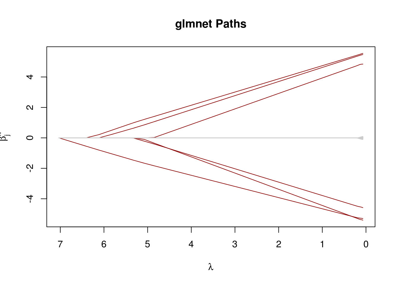
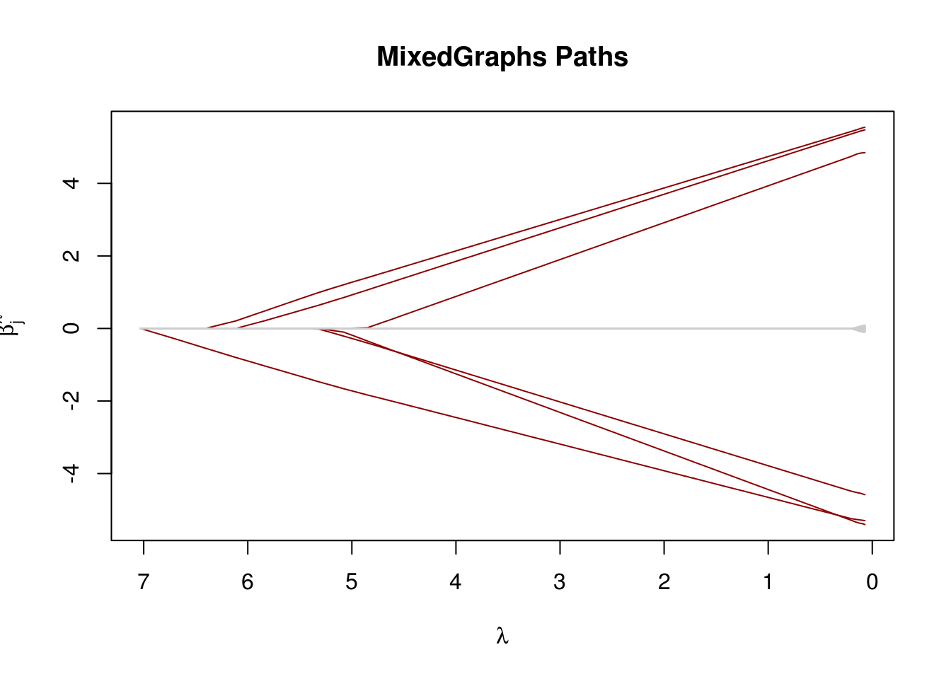
Compare with glmnet

library("glmnet")
library("MixedGraphs")
n <- 200; p <- 500
s <- 6; ## True sparsity

set.seed(1)
X <- matrix(rnorm(n * p), ncol=p)
beta <- rep(0, p)
beta[1:s] <- runif(s, 4, 6) * c(-1, 1)
y <- X %*% beta + rnorm(n)

glmnet_fit <- glmnet(X, y, standardize = FALSE)
glmLasso_fit <- glmLasso(X, y, lambda = glmnet_fit$lambda, support_stability = 10)